A simple traffic model

I have previously done some work with cell / compartment based modelling, so I guess I'll attempt to do a similar thing with traffic flows.

The model

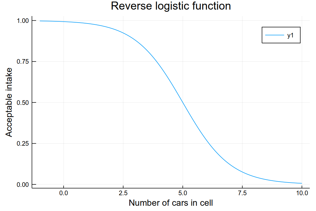
Each cell can be thought of as a segment of road. The outflow from each cell is based on the density of vehicles in the next cell. I think a logistic function here is a decent starting point.

using Plots
using DifferentialEquations

function reverseLogistic(x)
    # Logistic curve, scaled, shifted, and reversed.
    L = 1
    x₀ = -5
    k = 1
    
    return L / (1 + exp(-k * (-x - x₀)))
end
    
plot(-1:0.01:10, reverseLogistic, title="Reverse logistic function", xlabel="Number of cars in cell", ylabel="Acceptable intake")

Plot of the reverse logistic function from 0 to 10

It makes sense to me that the flux into the next cell is $v = \min(\text{stuff in current cell}, \text{intake allowed by adjacent cell})$, or $v(c_i, c_j)$.

Thus for some cell $c_i$, the simplest model I can think of looks like

$$ \frac{d}{dt} c_i(t) = v(c_{i-1}, c_i) - v(c_i, c_{i+1}) $$

The reverse logistic function provides a number of feature I'd like to have included in the model. For example, we can set a "carrying capacity", or a maximum number of cars in the cell. We can also adjust how fast flux in and out of the cell is. Roughly, these parameters correspond to the size of a road segment and its throughput. Obviously some parameter tuning will be needed so that things make proper sense, but that'll come later.

The model I have in mind for this blog post looks like this:

Sketch of the cell-based traffic model

Traffic flows from cell 1 to cell 2 to cell 3, and into a controlled intersection $I$, into cell 4, 5, etc.

The controlled intersection allows us to turn on and off the logistic function we are using for intake. In other words, at a red light, the cell doesn't accept any cars. At a green light, works like any other cell.

function heaviside(t, x)
    return t > 10 ? reverseLogistic(x) : 0
end

function simpletrafficmodel(dc, c,p,t)
    dc[1] = - min(c[1], reverseLogistic(c[2]))
    dc[2] = min(c[1], reverseLogistic(c[2])) - min(c[2], reverseLogistic(c[3]))
    dc[3] = min(c[2], reverseLogistic(c[3])) - min(c[3], heaviside(t,reverseLogistic(c[4])))
                # Use of heaviside function sets intake to 0 until t = 10
    dc[4] = min(c[3], heaviside(t,reverseLogistic(c[4]))) - min(c[4], reverseLogistic(c[5]))
    dc[5] = min(c[4], reverseLogistic(c[5])) - min(c[5], reverseLogistic(c[6]))
    dc[6] = min(c[5], reverseLogistic(c[6])) - min(c[6], reverseLogistic(c[7]))
    dc[7] = - min(c[7], 1)
end

c0 = [20.0; 0.0; 0.0; 0.0; 0.0; 0.0; 0.0]
tspan = (0.0, 30.0)
prob = ODEProblem(simpletrafficmodel, c0, tspan)
sol = solve(prob)

>>  retcode: Success
>>  Interpolation: Automatic order switching interpolation
>>  t: 46-element Array{Float64,1}:
>>    0.0                  
>>    0.0010066876113602205
>>    0.011073563724962425 
>>    0.06462164142708157  
>>    0.16697297707764686  
>>    0.3218211052641421   
>>    0.5355997770844789   
>>    0.8258553475334216   
>>    1.2034110867394991   
>>    1.6832643790417663   
>>    2.2771586701866986   
>>    3.0006153717003694   
>>    3.8727297491693498   
>>    ⋮                    
>>   16.3907327633898      
>>   17.505614833052345    
>>   18.826911298180665    
>>   20.31765405875277     
>>   22.268406351716       
>>   24.364818208663557    
>>   25.553796458452556    
>>   26.661460411536456    
>>   27.750085372546785    
>>   28.67308082944236     
>>   29.71635884247561     
>>   30.0                  
>>  u: 46-element Array{Array{Float64,1},1}:
>>   [20.0, 0.0, 0.0, 0.0, 0.0, 0.0, 0.0]                                 
>>   [19.999, 0.000999444, 5.03149e-7, 0.0, 0.0, 0.0, 0.0]                
>>   [19.989, 0.0109384, 6.06759e-5, 0.0, 0.0, 0.0, 0.0]                  
>>   [19.9358, 0.0621456, 0.00202975, 0.0, 0.0, 0.0, 0.0]                 
>>   [19.8342, 0.152662, 0.0131022, 0.0, 0.0, 0.0, 0.0]                   
>>   [19.6807, 0.273026, 0.0463031, 0.0, 0.0, 0.0, 0.0]                   
>>   [19.4689, 0.41113, 0.119962, 0.0, 0.0, 0.0, 0.0]                     
>>   [19.1818, 0.556737, 0.261459, 0.0, 0.0, 0.0, 0.0]                    
>>   [18.809, 0.692184, 0.498852, 0.0, 0.0, 0.0, 0.0]                     
>>   [18.3359, 0.8041, 0.86002, 0.0, 0.0, 0.0, 0.0]                       
>>   [17.7512, 0.884859, 1.36395, 0.0, 0.0, 0.0, 0.0]                     
>>   [17.0397, 0.935615, 2.0247, 0.0, 0.0, 0.0, 0.0]                      
>>   [16.1826, 0.985369, 2.83202, 0.0, 0.0, 0.0, 0.0]                     
>>   ⋮                                                                    
>>   [5.95265, 4.14148, 3.62996, 0.98074, 0.969976, 0.93652, 0.0]         
>>   [5.15709, 4.03118, 3.44064, 0.98199, 0.977505, 0.962471, 0.0]        
>>   [4.18196, 3.89692, 3.25209, 0.982158, 0.980783, 0.97536, 0.0]        
>>   [3.04251, 3.75017, 3.0739, 0.982252, 0.981629, 0.980445, 0.0]        
>>   [1.49678, 3.57268, 2.88085, 0.982302, 0.982095, 0.98194, 0.0]        
>>   [0.236829, 2.94416, 2.70997, 0.982318, 0.982258, 0.982248, 0.0]      
>>   [0.0722884, 2.0249, 2.62581, 0.982322, 0.982304, 0.982273, 0.0]      
>>   [0.0239105, 1.05687, 2.55413, 0.982323, 0.982316, 0.982299, 0.0]     
>>   [0.00805945, 0.289408, 2.26806, 0.982323, 0.982321, 0.982313, 0.0]   
>>   [0.00320327, 0.117975, 1.53767, 0.982323, 0.982322, 0.982318, 0.0]   
>>   [0.00112944, 0.042768, 0.670052, 0.902385, 0.982323, 0.982321, 0.0]  
>>   [0.000850509, 0.0324471, 0.513743, 0.823946, 0.952888, 0.978803, 0.0]

xs = ["$i" for i in 1:7]
ys = ["1"]
anim = @animate for i in 1:length(sol)
    heatmap(xs, ys, sol[i], clim=(0,10))
end
gif(anim)

An animation of the traffic model

This is basically what we'd expected: The number of cars from cells 1 leaks into cell 2 and 3, but there's a build up at cell 3, then at cell 2, because of a "red light". Once the light is green, traffic continues to flow through cells 4, 5, 6, 7.